Calculate the Kendrick mass defect (KMD) — calc

The Kendrick mass defect (KMD) is calculated by subtracting the Kendrick mass (calc_km) from the nominal Kendrick mass (calc_nominal_km). The the References section for more information.

Usage

calc_kmd(mass, repeating_unit = "CH2")

Arguments

mass: A molecular mass (or m/z).
repeating_unit: The formula of the repeating unit, given as a string.

Value

The Kendrick mass defect (KMD)

References

Kendrick mass on Wikipedia
Edward Kendrick, Anal. Chem. 1963, 35, 2146–2154.
C. A. Hughey, C. L. Hendrickson, R. P. Rodgers, A. G. Marshall, K. Qian, Anal. Chem. 2001, 73, 4676–4681.

Examples

# Calculate the Kendrick mass defects for two measured masses with
# CH2 as the repeating unit.
# See Hughey et al. in the References section above

calc_kmd(c(351.3269, 365.3425))
#> [1] 0.06539637 0.06544638

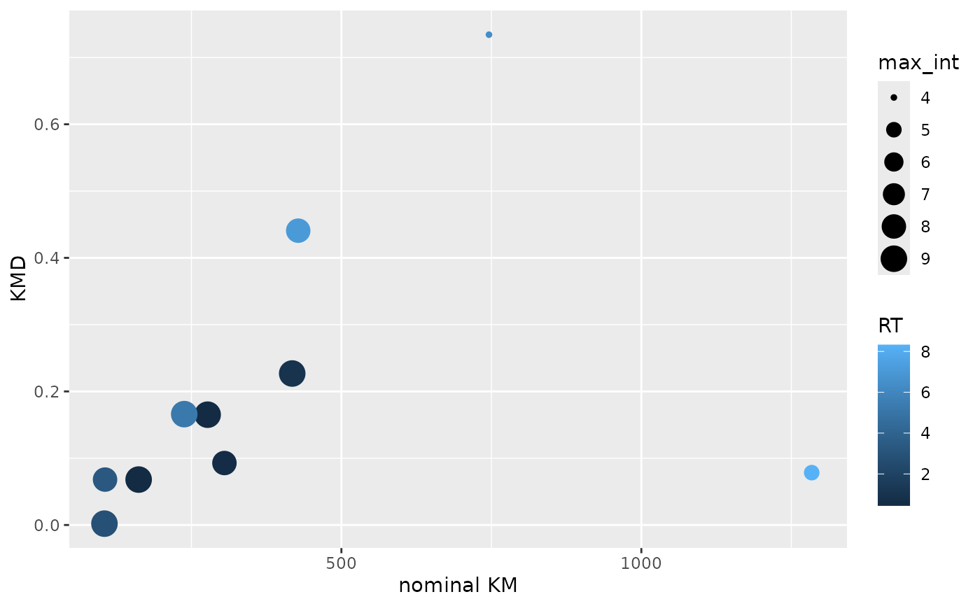
# Construct a KMD plot from m/z values.
# RT is mapped to color and the feature-wise maximum intensity to size.

toy_metaboscape %>%
  dplyr::group_by(UID, `m/z`, RT) %>%
  dplyr::summarise(max_int = max(Intensity, na.rm = TRUE)) %>%
  dplyr::ungroup() %>%
  dplyr::mutate(KMD = calc_kmd(`m/z`),
                `nominal KM` = calc_nominal_km(`m/z`)) %>%
  ggplot2::ggplot(ggplot2::aes(x = `nominal KM`,
                               y = KMD,
                               size = max_int,
                               color = RT)) +
    ggplot2::geom_point()
#> `summarise()` has grouped output by 'UID', 'm/z'. You can override using the
#> `.groups` argument.